How to Geo-Partition Data in Distributed SQL
How to achieve high performance and regulatory compliance with partitioning.
Join the DZone community and get the full member experience.
Join For FreeWe are excited to announce the availability of row-level geo-partitioning in YugabyteDB, a feature heavily requested by our user community and enterprise customers alike. This feature allows fine-grained control over pinning data in a user table (at a per-row level) to geographic locations, thereby allowing the data residency to be managed at the database level.
Making the nodes of a multi-region database cluster aware of the location characteristics of the data they store allows conforming to regulatory compliance requirements such as GDPR by keeping the appropriate subset of data local to different regions, and is arguably the most intuitive way to eliminate the high latency that would otherwise get incurred when performing operations on faraway, remote regions.
In keeping with our 100% open source ethos, this feature is available in YugabyteDB under the Apache 2.0 license, so you can try it out right from your laptop! This blog post will dive into the details of this feature such as the high-level design, use-case benefits, as well as the how to use it.
Why Geo-Partition Data?
Geo-partitioning of data is critical to some global applications. However, global applications are not deployed using one particular multi-region deployment topology. The multi-region deployment topologies could vary significantly depending on the needs of the application, some of which are very common and critical.
In order to understand why geo-partitioning is useful, it is necessary to understand some of these deployment topologies, which are summarized in the table below.
| Synchronous multi-region | Asynchronous multi-region |
Geo-partitioned multi-region |
|
|---|---|---|---|
| Data replication across geographies | All data replicated across regions | All data replicated inside region, some data replicated across regions | Data partitioned across regions, partitions replicated inside region |
| Latency of queries from different regions | High | Low | Low |
| Consistency semantics | Transactional | Eventual consistency | Transactional |
| Schema changes across regions | Transparently managed | Manually propagated | Transparently managed |
| Data loss on region failure | None | Some data loss | No data loss (partial unavailability is possible) |
As seen from the table above, geo-partitioning can satisfy use cases that need low latencies without sacrificing transactional consistency semantics and transparently perform schema changes across the regions. Geo-partitioning makes it easy for developers to move data closer to users for lower latency, higher performance, and meeting data residency requirements to comply with regulations such as GDPR.
How Does It Work?
Geo-partitioning of data enables fine-grained, row-level control over the placement of table data across different geographical locations. This is accomplished in two simple steps – first, partitioning a table into user-defined table partitions, and subsequently pinning these partitions to the desired geographic locations by configuring metadata for each partition.
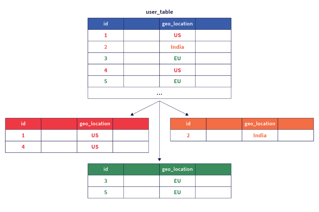
The first step of creating user-defined table partitions is done by designating a column of the table as the partition column that will be used to geo-partition the data. The value of this column for a given row is used to determine the table partition that the row belongs to. The figure below shows this.
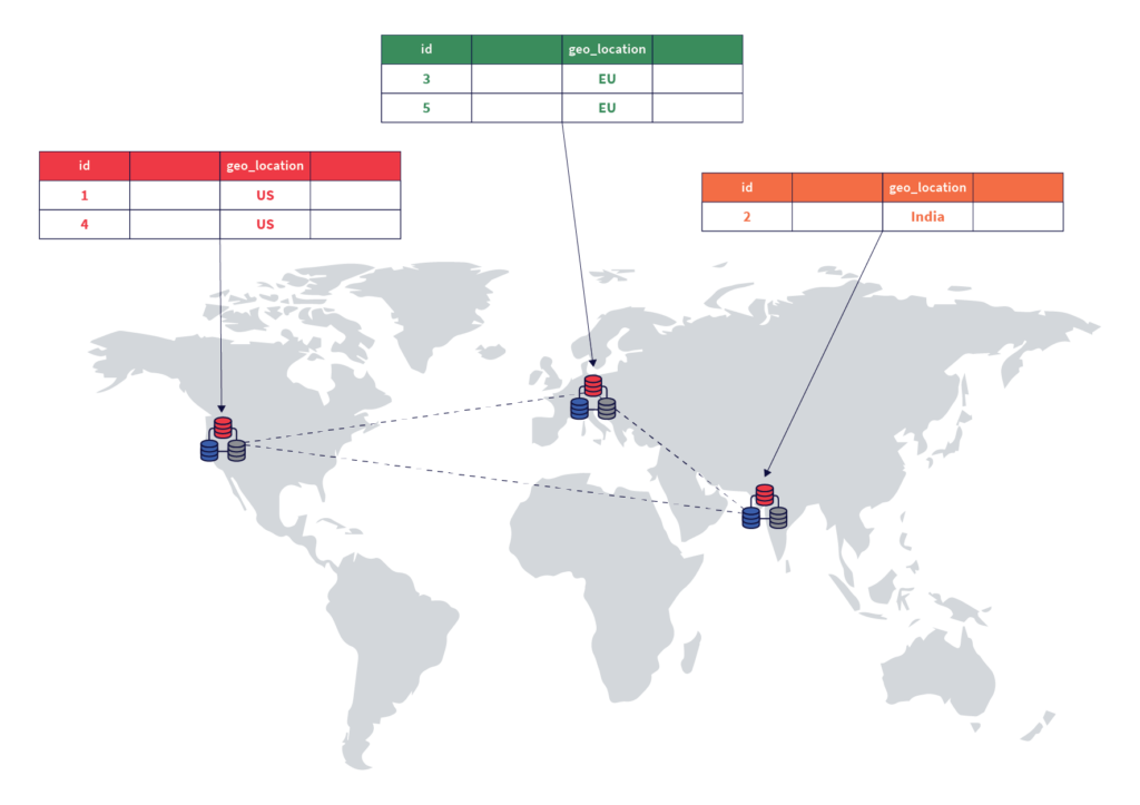
The second step involves configuring the partitions created in step one to pin data to the respective geographic locations by setting the appropriate metadata. Note that the data in each partition can be configured to get replicated across multiple zones in a cloud provider region, or across multiple nearby regions / datacenters.
An entirely new geographic partition can be introduced dynamically by adding a new table partition and configuring it to keep the data resident in the desired geographic location. Data in one or more of the existing geographic locations can be purged efficiently simply by dropping the necessary partitions. Users of traditional RDBMS would recognize this scheme as being close to user-defined list-based table partitions, with the ability to control the geographic location of each partition.
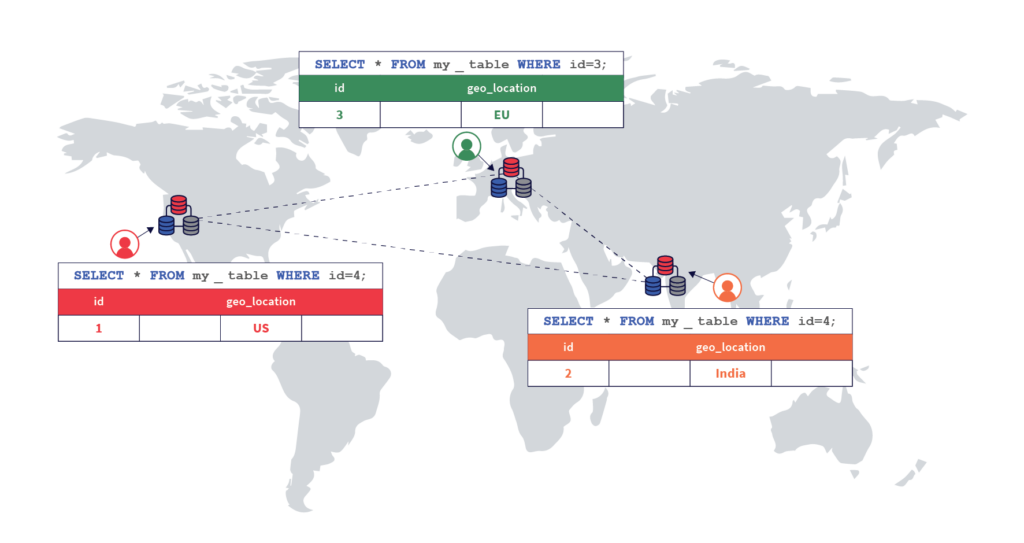
In this deployment, users can access their data with low latencies because the data resides on servers that are geographically close by, and the queries do not need to access data in far away geographic locations. This is shown in the diagram below.
Example Scenario
Let us look at this feature in the context of a use case. Say that a large but imaginary bank, Yuga Bank, wants to offer an online banking service to users in many countries by processing their deposits, withdrawals, and transfers. The following attributes would be required in order to build such a service.
- Transactional semantics with high availability: Consistency of data is paramount in a banking application, hence the database should be ACID compliant. Additionally, users expect the service to always be available, making high availability and resilience to failures a critical requirement.
- High performance: The online transactions need to be processed with a low latency in order to ensure a good end-user experience. This requires that the data for a particular user is located in a nearby geographic region. Putting all the data in a single location in an RDBMS would mean the requests for users residing far away from that location would have very high latencies, leading to a poor user experience.
- Data residency requirements for compliance: Many countries have regulations around which geographic regions the personal data of their residents can be stored in, and bank transactions being personal data are subject to these requirements. For example, GDPR has a data residency stipulation which effectively requires that the personal data of individuals in the EU be stored in the EU. Similarly, India has a requirement issued by the Reserve Bank of India (or RBI for short) making it mandatory for all banks, intermediaries, and other third parties to store all information pertaining to payments data in India – though in case of international transactions, the data on the foreign leg of the transaction can be stored in foreign locations.
Pitfalls of the Traditional “One Database Per Region” Approach
It is possible to deploy and manage independent relational databases in the different geographic regions, each storing the data for the appropriate set of users to achieve both data locality and compliance with regulatory requirements. The disadvantages of such an approach are:
- Since a given user can travel and perform transactions from different geographic regions, the data for that user can get fragmented over different independent databases over time. Operations such as viewing the transaction history for a user can get hard to implement.
- Additionally, the application would need to encode the database deployment topology in order to connect to the correct set of databases for a given user, and would need to be constantly updated as the deployment topology changes. This can make the application development very complex.
- Ensuring high availability and scalability of multiple single-node RDBMS in production databases is operationally very hard and error prone.
Using Geo-Partitioning for the Example Scenario
In the geo-partitioning approach, we simply deploy one YugabyteDB cluster across the different regions and create a geo-partitioned table for storing the user transactions as shown below.
Step 1. Create the Parent Table and Partitions
First, we create the parent table that contains a geo_partition column which is used to create list-based partitions for each geographic region we want to partition data into.
CREATE TABLE transactions (
user_id INTEGER NOT NULL,
account_id INTEGER NOT NULL,
geo_partition VARCHAR,
account_type VARCHAR NOT NULL,
amount NUMERIC NOT NULL,
txn_type VARCHAR NOT NULL,
created_at TIMESTAMP DEFAULT NOW()
) PARTITION BY LIST (geo_partition);
Next, we create one partition per desired geography under the parent table. In the example below, we create three table partitions – one for the EU region called transactions_eu, another for the India region called transactions_india, and a third default partition for the rest of the regions called transactions_default.
xxxxxxxxxx
CREATE TABLE transactions_eu
PARTITION OF transactions
(user_id, account_id, geo_partition, account_type,
amount, txn_type, created_at,
PRIMARY KEY (user_id HASH, account_id, geo_partition))
FOR VALUES IN ('EU');
CREATE TABLE transactions_india
PARTITION OF transactions
(user_id, account_id, geo_partition, account_type,
amount, txn_type, created_at,
PRIMARY KEY (user_id HASH, account_id, geo_partition))
FOR VALUES IN ('India');
CREATE TABLE transactions_default
PARTITION OF transactions
(user_id, account_id, geo_partition, account_type,
amount, txn_type, created_at,
PRIMARY KEY (user_id HASH, account_id, geo_partition))
DEFAULT;
Note that these statements above will create the partitions, but will not pin them to the desired geographical locations. This is done in the next step. The table and partitions created so far can be viewed using the \d command.
xxxxxxxxxx
yugabyte=# \d
List of relations
Schema | Name | Type | Owner
--------+----------------------+-------+----------
public | transactions | table | yugabyte
public | transactions_default | table | yugabyte
public | transactions_eu | table | yugabyte
public | transactions_india | table | yugabyte
(4 rows)
Step 2. Pin Partitions to Geographic Locations
Now that we have a table with the desired three partitions, the final step is to pin the data of these partitions to the desired geographical locations. In the example below, we are going to use regions and zones in the AWS cloud.
First, we pin the data of the EU partition transactions_eu to live across three zones of the Europe (Frankfurt) region eu-central-1 as shown below.
xxxxxxxxxx
$ yb-admin --master_addresses <yb-master-addresses> \
modify_table_placement_info ysql.yugabyte transactions_eu \
aws.eu-central-1.eu-central-1a,aws.eu-central-1.eu-central-1b,\
... 3
Second, we pin the data of the India partition transactions_india to live across three zones in India – Asia Pacific (Mumbai) region ap-south-1 as shown below.
xxxxxxxxxx
$ yb-admin --master_addresses <yb-master-addresses> \
modify_table_placement_info ysql.yugabyte transactions_india \
aws.ap-south-1.ap-south-1a,aws.ap-south-1.ap-south-1b,... 3
Finally, pin the data of the default partition transactions_default to live across three zones in the US West (Oregon) region us-west-2. This is shown below.
xxxxxxxxxx
$ yb-admin --master_addresses <yb-master-addresses> \
modify_table_placement_info ysql.yugabyte transactions_default \
aws.us-west-2.us-west-2a,aws.us-west-2.us-west-2b,... 3
Step 3. Pinning User Transactions to Geographic Locations
Now, the setup should automatically be able to pin rows to the appropriate regions based on the value set in the geo_partition column. Let us test this by inserting a few rows of data and verifying they are written to the correct partitions.
First, we insert a row into the table with the geo_partition column value set to EU below.
xxxxxxxxxx
INSERT INTO transactions
VALUES (100, 10001, 'EU', 'checking', 120.50, 'debit');
All of the rows above should be inserted into the transactions_eu partition, and not in any of the others. We can verify this as shown below. Note that we have turned on the expanded auto mode output formatting for better readability by running the statement shown below.
xxxxxxxxxx
yugabyte=# \x auto
Expanded display is used automatically.
The row must be present in the transactions table, as seen below.
xxxxxxxxxx
yugabyte=# select * from transactions;
-[ RECORD 1 ]-+---------------------------
user_id | 100
account_id | 10001
geo_partition | EU
account_type | checking
amount | 120.5
txn_type | debit
created_at | 2020-11-07 21:28:11.056236
Additionally, the row must be present only in the transactions_eu partition, which can be easily verified by running the select statement directly against that partition. The other partitions should contain no rows.
xxxxxxxxxx
yugabyte=# select * from transactions_eu;
-[ RECORD 1 ]-+---------------------------
user_id | 100
account_id | 10001
geo_partition | EU
account_type | checking
amount | 120.5
txn_type | debit
created_at | 2020-11-07 21:28:11.056236
yugabyte=# select count(*) from transactions_india;
count
-------
0
yugabyte=# select count(*) from transactions_default;
count
-------
0
Now, let us insert data into the other partitions.
xxxxxxxxxx
INSERT INTO transactions
VALUES (200, 20001, 'India', 'savings', 1000, 'credit');
INSERT INTO transactions
VALUES (300, 30001, 'US', 'checking', 105.25, 'debit');
These can be verified as shown below.
xxxxxxxxxx
yugabyte=# select * from transactions_india;
-[ RECORD 1 ]-+---------------------------
user_id | 200
account_id | 20001
geo_partition | India
account_type | savings
amount | 1000
txn_type | credit
created_at | 2020-11-07 21:45:26.011636
yugabyte=# select * from transactions_default;
-[ RECORD 1 ]-+---------------------------
user_id | 300
account_id | 30001
geo_partition | US
account_type | checking
amount | 105.25
txn_type | debit
created_at | 2020-11-07 21:45:26.067444
Step 4. Users Traveling Across Geographic Locations
In order to make things interesting, let us say user 100, whose first transaction was performed in the EU region travels to India and the US, and performs two other transactions. This can be simulated by using the following statements.
xxxxxxxxxx
INSERT INTO transactions
VALUES (100, 10001, 'India', 'savings', 2000, 'credit');
INSERT INTO transactions
VALUES (100, 10001, 'US', 'checking', 105, 'debit');
Now, each of the transactions would be pinned to the appropriate geographic locations. This can be verified as follows.
xxxxxxxxxx
yugabyte=# select * from transactions_india where user_id=100;
-[ RECORD 1 ]-+---------------------------
user_id | 100
account_id | 10001
geo_partition | India
account_type | savings
amount | 2000
txn_type | credit
created_at | 2020-11-07 21:56:26.760253
yugabyte=# select * from transactions_default where user_id=100;
-[ RECORD 1 ]-+---------------------------
user_id | 100
account_id | 10001
geo_partition | US
account_type | checking
amount | 105
txn_type | debit
created_at | 2020-11-07 21:56:26.794173
All the transactions made by the user can efficiently be retrieved using the following SQL statement.
xxxxxxxxxx
yugabyte=# select * from transactions where user_id=100 order by created_at desc;
-[ RECORD 1 ]-+---------------------------
user_id | 100
account_id | 10001
geo_partition | US
account_type | checking
amount | 105
txn_type | debit
created_at | 2020-11-07 21:56:26.794173
-[ RECORD 2 ]-+---------------------------
user_id | 100
account_id | 10001
geo_partition | India
account_type | savings
amount | 2000
txn_type | credit
created_at | 2020-11-07 21:56:26.760253
-[ RECORD 3 ]-+---------------------------
user_id | 100
account_id | 10001
geo_partition | EU
account_type | checking
amount | 120.5
txn_type | debit
created_at | 2020-11-07 21:28:11.056236
Step 5. Adding a New Geographic Location
Assume that after a while, our fictitious Yuga Bank gets a lot of customers across the globe, and wants to offer the service to residents of Brazil, which also has data residency laws. Thanks to row-level geo-partitioning, this can be accomplished easily. We can simply add a new partition and pin it to the AWS South America (São Paulo) region sa-east-1 as shown below.
xxxxxxxxxx
CREATE TABLE transactions_brazil
PARTITION OF transactions
(user_id, account_id, geo_partition, account_type,
amount, txn_type, created_at,
PRIMARY KEY (user_id HASH, account_id, geo_partition))
FOR VALUES IN ('Brazil');
$ yb-admin --master_addresses <yb-master-addresses> \
modify_table_placement_info ysql.yugabyte transactions_brazil \
aws.sa-east-1.sa-east-1a,aws.sa-east-1.sa-east-1b,... 3
And with that, the new region is ready to store transactions of the residents of Brazil.
xxxxxxxxxx
INSERT INTO transactions
VALUES (400, 40001, 'Brazil', 'savings', 1000, 'credit');
yugabyte=# select * from transactions_brazil;
-[ RECORD 1 ]-+-------------------------
user_id | 400
account_id | 40001
geo_partition | Brazil
account_type | savings
amount | 1000
txn_type | credit
created_at | 2020-11-07 22:09:04.8537
Conclusion
The YugabyteDB 2.5 release adds row-level geo-partitioning capabilities, a very critical feature that enables some key use-cases, along with follower reads to the already extensive set of multi-region features in YugabyteDB. These new features, combined with the ability to perform synchronous replication across 3 or more regions and asynchronous replication across 2 or more regions (called xCluster replication), makes YugabyteDB the distributed SQL database with the most comprehensive set of multi-region deployment options. These deployment options across multiple data centers, regions and/or clouds give users even more control to bring data close to their customers for performance, costs, or compliance reasons. All of the features mentioned are 100% open source under the Apache v2 license.
Opinions expressed by DZone contributors are their own.
Comments